Notes on LLM technologies (keep updating)
LLM techTable of Contents
Brief notes on LLM technologies.
Models
GPT2
Model structure
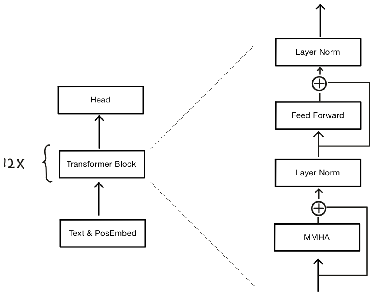
The GPT model employs a repeated structure of Transformer Blocks, each containing two sub-layers: a Masked Multi-Head Attention (MMHA) layer and a Position-wise Feed-Forward Network.
The MMHA is a central component of the model. It operates by splitting the input into multiple ‘heads’, each of which learns to attend to different positions within the input sequence, allowing the model to focus on different aspects of the input simultaneously. The output of these heads is then concatenated and linearly transformed to produce the final output.
The MMHA mechanism can be formally defined as follows:
\[ MultiHead(Q,K,V) = Concat(head_1, \cdots, head_h)W^O \]
where each head is computed as:
\[ head_i = Attention(QW_i^Q, KW_i^K, VW_i^V) \]
In implementation, the computation of \(Q,K,V\) can be packed together with Linear operations regardless of the number of heads, like
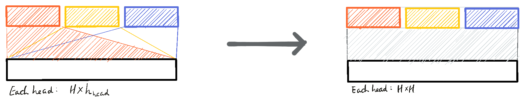
And the computation is as below
\begin{split} Q &= xW^Q \\ K &= xW^K \\ V &= xW^V \end{split}
The Attention function is defined as:
\[ Attention(q_i, k_i, v_i) = softmax(\frac{q_i k_i^T}{\sqrt{d_k}})v_i \]
Here, \(d_k\) represents the dimension of the keys, which is calculated as \(d_k = \frac{H}{h}\), where \(H\) is the total dimension of the input and \(h\) is the number of heads.
To ensure the MHA mechanism works correctly with sequences of varying lengths, a Mask is applied. This Mask effectively ignores padding elements by setting their values to \(-\infty\), allowing the Softmax function to handle them appropriately. The layer output demensions are as below:
| Layer | Dimensions | Note |
|---|---|---|
| Model input | [bs, seq_len] | Token IDs |
| Text & PosEmbed | [bs, seq_len, H] | Text embeddings + position embeddings |
| Layer Norm (0) | [bs, seq_len, H] | |
| Feed Forward | [bs, seq_len, H] | |
| Layer Norm (1) | [bs, seq_len, H] | |
| \(head_i\) | [bs, seq_len, H/h] | |
| MMHA | [bs, seq_len, H] |
Where
bsis the batch sizeseq_lenis the max length of the sequenceHis the size of the hidden statehis the number of heads
Reference
- Leviathan, Yaniv, Matan Kalman, and Yossi Matias. “Fast inference from transformers via speculative decoding.” International Conference on Machine Learning. PMLR, 2023.
- Multi-head attention in Pytorch
Lora
Algorithm
 (image borrowed from this page)
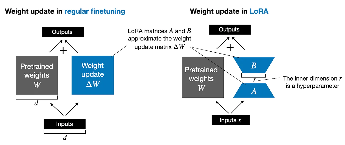
A classical workflow to finetune an LLM is to learn an additional parameters denoted as \(\delta W\) as long as frooze the original parameters, just as the left part of the figure below.
\[ h = W_0 x \Rightarrow (W_0 + \delta W) x \]
This could be applied on the \(W_q, W_k, W_v\) and \(W_o\) in the Transformer block, while since the Transformer blocks contains the mojority of the parameters, that workflow could result in significant increase of additional parameters.
For instance, a Llama V1 7B model, whose hidden size is 4096, and the dimension of the MLP’s inner layer is 11008, let’s zoom into a Transformer layer, the \(W_q, W_k, W_v, W_o\), each contains \(4096 \times 4096 = 4096 \times 128=16.78M\) parameters, and the MLP contains three Linear layer of \(135.27M\) parameters, and two RMSNorm layers each contains \(4096=4M\) parameters. In total, a single Transformer layer contains \(16.78M \times 4 + 135.27M + 4M\times 2=210.29M\). You can refer to Superjomn’s blog | Count the parameters in LLaMA V1 model for details about counting the parameters.
The LoRA is for such scenarios, instead of learning the \(\delta W\) itself, it learns decomposed representation of \(\delta W\) directly during finetune training. Since the rank could be \(8\), that could reduce the number of trainable parameters required for adaptation to downstream tasks. Let’s revisit the Llama V1 7B example, if we apply LoRA on all the Linear layers within a Transformer layer:
- \(W_q, W_k, W_v, W_o\) each will take \(4096*8 + 8*4096=0.065M\) parameters
- MLP have \(3 \times (4096 \times 8 + 8 \times 11008)=0.362M\)
So in total, the LoRA will bring \(0.362+0.065*4=0.622\) additional parameters, that is only \(\frac{0.622}{210.29}=0.29\%\) of the original parameters.
So instead of fully-finetune all the original paramters, the LoRA could finetune the LLaMA 7B model with less than 1% parameters, that is quite efficient.
Reference
- Practical Tips for Finetuning LLMs Using LoRA (Low-Rank Adaptation)
- Hu, Edward J., et al. “Lora: Low-rank adaptation of large language models.” arXiv preprint arXiv:2106.09685 (2021).
Speculative decoding
Motivation
Consider a scenerio where we have a prefix such as “Geoffrey Hinton did his PhD at the University”, and the target suffix is “of Edinburgh”. When a LLM continues the generation, it is evident that:
- The word “of” is simple to generate and could be produced by a smaller model given the same prefix
- The word “Edinburgh” is more challenging to generate and may require a larger model with more knowledge
Speculative decoding addresses this by using a smaller model to generate “easy” words like “of” for better throughput, while leaving more challenging words to a larger model for precision.
Algorithm
Speculative decoding employs two models:
- A draft model, denoted as \(M_p\), which is smaller and much faster (as least 2X) to give a sub-sequence of the next K tokens.
- A target model, denoted as \(M_q\), which is larger and more precise. It evaluates the sub-sequence generated by the draft model.
Assuming K to be 4, the prefix to be \(pf\), and the draft model generates five tokens based on \(pf\):
- Token \(x_1\), the probability is \(p_1(x) = M_p(pf)\)
- Token \(x_2\) with probability of \(p_2(x) = M_p(pf, x_1)\)
- Token \(x_3\) with probability of \(p_3(x) = M_p(pf, x_1, x_2)\)
- Token \(x_4\) with probability of \(p_4(x) = M_p(pf, x_1, x_2, x_3)\)
The target model evalutes K tokens generated by \(M_p\) with a single model forward pass, similar to the training phase:
\[ q_1(x), q_2(x), q_3(x), q_4(x) = M_q(pf, x_1, x_2, x_3, x_4) \]
Let’s consider a real example to illustrate the heuristics. Suppose the draft model generate the following sub-sequence with \(K=4\):
| Token | x1 | x2 | x3 | x4 |
|---|---|---|---|---|
| dogs | love | chasing | after | |
| p(x) | 0.8 | 0.7 | 0.9 | 0.8 |
| q(x) | 0.9 | 0.8 | 0.8 | 0.3 |
| q(x)>=p(x)? | Y | Y | N | N |
| accept prob | 1 | 1 | 0.8/0.9 | 0.3/0.8 |
The rules is as below:
- If \(q(x) >= p(x)\), then accept the token.
- If not, the accept probability is \(\frac{q(x)}{p(x)}\), so the token “chasing” has a probability of \(\frac{0.8}{0.9}=89\%\), while the next token “after” has an accept probability of only \(\frac{0.3}{0.8}=37.5\%\).
- If a word is unaccepted, the candidate word after it will be dropped as well. It will be resampled by target model, not the draft model.
- Repeat the steps above from the next position
Reference
Speculative Decoding: When Two LLMs are Faster than One - YouTube